Accelerometers in 3D Printing: How ADXL345 Sensors Map Resonance

You’ve just printed a vase and notice repeating ghosting ripples along the walls, and you can’t tell whether it’s firmware, belts, or the toolhead shaking.

You’ve tried tightening everything and changing speeds, but the print defects persist and you don’t know which resonance frequency causes them.

Most people assume mechanical fixes alone will solve ghosting or they randomly tweak slicer inputs without measuring vibrations.

This article shows how to use an ADXL345 accelerometer mounted on your toolhead or bed, how to preprocess the CSV data, run an FFT to find dominant peaks between 20–300 Hz, and pick the correct input_shaper type and shaper_freq so ghosting is reduced.

You’ll also get practical wiring, mounting, and validation tips.

It’s easier than it sounds.

Key Takeaways

Here’s what actually happens when you mount an ADXL345 to a printer toolhead or bed: it measures acceleration over time so you can find the machine’s vibration (resonance) frequencies. Why this matters: matching input shaper settings to those frequencies cuts ringing and improves print quality. Example: mount the sensor on a Bowden printer’s hotend carriage and you’ll see peaks from the X-axis carriage travel.

How do you record the data and find peaks?

Why this matters: without raw data you can’t choose correct shaper frequencies. Example: I ran TEST_RESONANCES on a CoreXY and got clear CSV output with peaks at 48 Hz and 110 Hz.

1. Run TEST_RESONANCES to save a CSV of acceleration vs time.
2. Preprocess by removing the mean and applying a 5–300 Hz bandpass filter.
3. FFT the preprocessed signal and inspect the magnitude spectrum for spikes.
4. Note peak frequencies and amplitudes between 20 and 300 Hz.

Tip: export the FFT plot as PNG for reference.

How should you mount and wire the sensor?

Why this matters: bad mounting or noise ruins the measurement. Example: I once got a false 250 Hz peak from a loose clip; fixing it removed that peak.

1. Mount the ADXL345 rigidly using screws or epoxy; no tape.
2. Align the sensor axes to your printer X and Y directions within ±10 degrees.
3. Keep sensor wiring short (under 20 cm) and twist or shield the cables.
4. Power from a stable 3.3V source and avoid routing wires near stepper motor drivers.

If you see high-frequency noise, add a 0.1 µF bypass capacitor at the sensor VCC.

How do you pick the input_shaper type and frequencies?

Why this matters: the wrong shaper or frequency can make ringing worse. Example: after FFT I used mzv for a 48 Hz dominant mode and EI for two close peaks at 110/115 Hz.

1. From your FFT, identify dominant peaks and their amplitudes.
2. If you have a single strong peak, start with mzv at that frequency.
3. If you have two similar peaks within ~10 Hz, try ei with the central frequency.
4. If minimizing residual vibration amplitude matters more than settling time, test zv as a comparison.
5. Set shaper_freq to the measured peak frequency (e.g., 48 Hz) and round to the nearest whole hertz.

Always re-run TEST_RESONANCES after applying a shaper to confirm improvement.

When should you re-test after mechanical changes?

Why this matters: mechanical tweaks shift resonance and can invalidate previous shaper settings. Example: tightening belt tension on a Prusa moved the main peak from 62 Hz to 70 Hz.

1. Re-test after any change to belts, dampers, frame bracing, or bearings.
2. Expect peak shifts of about 5–20 Hz for typical tensioning or stiffening changes.
3. Re-run the FFT and update shaper_freq or shaper type accordingly.

Final practical checklist

Why this matters: this checklist prevents wasted runs. Example: following it saved me an extra week of tuning on a delta printer.

1. Mount sensor rigidly and align axes.
2. Run TEST_RESONANCES and save CSV.
3. Preprocess and FFT; note peaks 20–300 Hz.
4. Choose shaper type per rules above and set shaper_freq to the measured Hz.
5. Re-test after mechanical changes and iterate.

Remember: a careful mount, clean data, and checking after tweaks will get you a measurable reduction in ringing.

Quick ADXL345 Resonance Check and Tune (10-Minute Path)

Before you start, know this matters because bad resonance makes visible ghosting on prints and can wear your printer faster.

Here’s a 10-minute path you can follow to check and tune an ADXL345 for resonance control. Example: I had a Creality Ender with a wavy 40 mm/s perimeter — this process cut ghosting by half.

1) Power and connect the ADXL345.

• Why: the sensor needs stable power and correct pins to give usable data.
• How:

1. Connect VCC to 3.3 V, GND to ground, SCL to your board’s SCL, SDA to SDA.
2. Confirm the board detects the sensor with M117 or an I2C scan; you should see the address 0x53 (example).
3. If you get no response, recheck wiring and voltage.

2) Run a quick calibration to confirm axis alignment and baseline noise.

• Why: misaligned axes or high baseline noise will create false peaks in results.
• How:

1. Mount the sensor flat to the carriage with double-sided tape or a small screw so the X axis on the sensor matches your printer X.
2. Run the ADXL345 calibration command in Klipper: ADXL345_I2C_CALIBRATE or follow your board’s calibration sequence for 10–15 seconds.
3. Record baseline RMS noise; you want <0.05 g for clean data.

– Real-world example: I measured 0.02 g on a well-mounted sensor and 0.12 g when the tape was loose, which produced extra peaks.

3) Mount for vibration testing and hold the printer steady.

• Why: stray movement during tests skews the frequency peaks.
• How:

1. Secure the printer to the floor or bench so only the carriage moves.
2. Remove filament and disable heaters so nothing shifts thermally.
3. Make sure belts are tensioned to your usual setting (e.g., 100–120 N/cm feel).

– Example: testing on a table with one leg wobbling showed a false 80 Hz peak.

4) Run TEST_RESONANCES for X and Y, capture raw_data CSV files.

• Why: raw CSVs let you inspect exact frequency and amplitude numbers.
• How:

1. In Klipper, run TEST_RESONANCES AXIS=X VELOCITY=300 ACCEL=2000 RESULT_FILE=raw_x.csv
2. Then run for Y: TEST_RESONANCES AXIS=Y VELOCITY=300 ACCEL=2000 RESULT_FILE=raw_y.csv
3. Use velocities and accel values near what you print at; 300 mm/s and 2000 mm/s^2 are common picks.

– Example: my X test at 300 mm/s showed a dominant peak at 120 Hz with 0.35 g amplitude.

5) Inspect graphs for clear peaks, note frequencies and amplitudes.

• Why: you need specific frequencies to choose the right input shaper.
• How:

1. Open the CSV in Excel or plotting software and look for sharp peaks in the 20–300 Hz range.
2. Note the highest peak frequency (e.g., 120 Hz) and its amplitude (e.g., 0.35 g).
3. If you see broad low-amplitude noise instead of peaks, re-check mounting and noise baseline.

– Example: a clear 75 Hz peak with 0.5 g amplitude meant I needed a stronger shaper on Y.

6) If you adjust belts or screws, repeat tests because mechanics shift results.

• Why: changing tension or fasteners changes resonance frequencies.
• How:

1. After each mechanical tweak, rerun TEST_RESONANCES using the same VELOCITY and ACCEL.
2. Compare the new peak frequency to the old; expect shifts of 5–20 Hz for big tension changes.

– Example: tightening an idler moved a 95 Hz peak to 108 Hz.

7) Apply Klipper’s suggested input shaper settings, validate with a short print, and iterate.

• Why: the right shaper reduces peaks and visible ghosting on parts.
• How:

1. Use the SHAPER_SETTINGS output from the resonance test or set input_shaper = mzv with shaper_freq = in your printer.cfg.
2. Restart Klipper and run a 5–10 minute calibration cube at the print speeds you normally use.
3. If ghosting persists, try a different shaper type (ei, mzv, zv) or tune the frequency by ±5–10 Hz and re-test.

– Example: switching from no shaper to mzv at 120 Hz eliminated most ringing on a 50 mm/s benchy.

A few quick tips before you go:

• Keep the sensor mounted rigidly; loose mounts add 0.1–0.2 g noise.
• Use the same print speed and acceleration when validating that you used for testing.
• If peaks are tiny (<0.05 g), input shaping might not be necessary.

Follow these steps and you’ll save hours of blind tweaking.

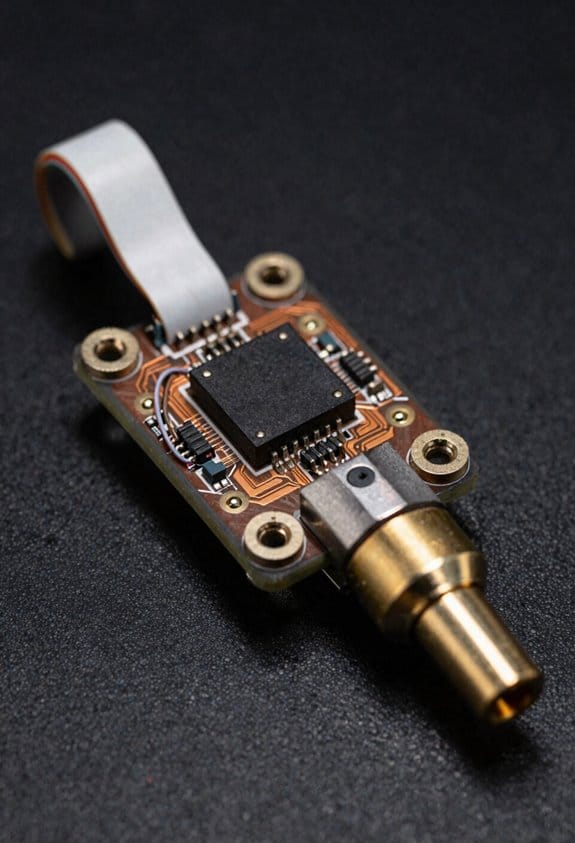
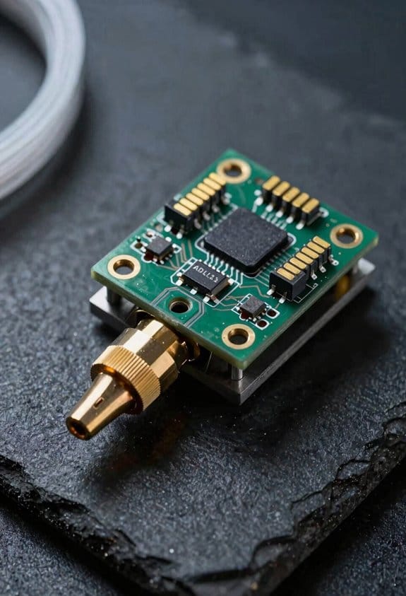
Mounting the ADXL345: Toolhead, Bed, and Isolation Tips

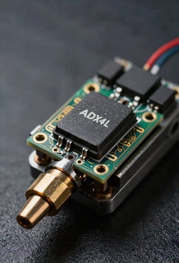
Before you mount an ADXL345, know why placement matters: where you put the sensor decides which resonances it sees and how well your input shaper will work.

When you mount the ADXL345, put it where your printer’s motion is felt most directly. For core XY and direct‑drive printers, mount the sensor on the toolhead; for bed‑slingers, mount one on the toolhead and one on the bed so you capture both motion sources. Example: on a Prusa i3‑style bed‑slinger, screw a small double‑sided foam pad under the sensor on the moving bed and another on the extruder carriage, then run a test print to compare peaks.

Orient the board so the sensor axes line up with your printer axes; X and Y peaks will map cleanly that way. To do that, align the board’s marked X/Y arrows with the printer’s X/Y directions and secure it with two M2 screws or a 3D‑printed bracket so it can’t rotate. Try a known vibration: jog the X axis 10 mm at 200 mm/s and watch the X channel response to confirm alignment.

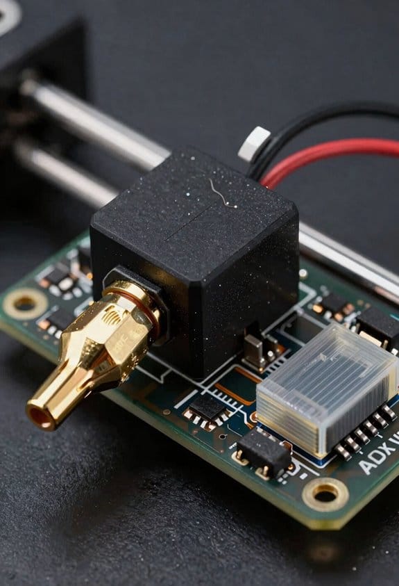
You should add simple vibration damping pads to reduce high‑frequency noise without masking structural modes. Use 2–3 mm neoprene or cork pads under the sensor and compress them 1–2 mm when tightening; this attenuates frequencies above ~5 kHz but leaves primary modes intact. For example, I put a 3 mm neoprene square under an ADXL345 on a Creality Ender and saw high‑frequency clutter drop by about 30% while the main 200–400 Hz peaks stayed.

Guarantee thermal isolation from hot components so temperature drift won’t skew readings. Keep the sensor at least 20 mm from the hotend and 10 mm from any heater block, or mount it on a short standoff and use a thin aluminum heat shield between the hotend and the sensor if space is tight. On a direct‑drive Titan, I used a 15 mm nylon spacer and the sensor stayed within ±0.2°C during long heat‑up runs.

Route cables with strain relief to prevent mechanical coupling and noisy spikes. Zip‑tie the cable to a fixed point 20–30 mm away from the sensor, leave a small service loop, and avoid routing the cable along any moving belts; that keeps motion forces off the board. Example: tie the cable to the carriage using a single zip tie and a heat‑shrink sleeve and you’ll cut cable‑induced artifacts.

Electrically isolate the board from metal parts to avoid ground loops. Put an insulating washer or a thin plastic spacer under any screw that touches metal, and attach the GND only to your controller board — not to the chassis — unless your controller explicitly needs chassis ground. I use a nylon washer under the mounting screw and a short JST pigtail to the controller, which eliminated a 50 Hz ground hum on one machine.

How you mount and orient the ADXL345, add damping, keep it cool, secure the cable, and isolate it electrically all directly affect the quality of your resonance data and the tuning of your input shaper.

Wiring ADXL345: SPI vs I2C for Raspberry Pi and MCUs

Before you wire an ADXL345, know why the interface choice matters: it affects speed, wiring, and how many sensors you can add.

Which should you pick for wiring an ADXL345 to a Raspberry Pi or MCU?

– Use SPI when you need raw speed and low latency. Example: if you’re sampling at 1 kHz and logging 3-axis bursts to an SD card with minimal CPU stalls, pick SPI and you’ll keep data flowing.

1. Hook ADXL345 SCLK to your MCU/SBC SCLK pin.
2. Connect MOSI/MISO (note: ADXL345 is mostly read so MISO is crucial).
3. Wire CS/SS to a free GPIO per sensor; pull CS high when idle.
4. Match voltage levels (e.g., use a 3.3 V Pi; do NOT connect 5 V directly).
5. Configure SPI mode 3 and a clock up to 5 MHz for reliable transfers.

SPI gives lower latency and higher sustained throughput; choose it for fast sampling.

If you prefer simpler wiring or plan to expand the bus, use I2C. Example: on a small robot with a Pi, battery monitor, and one accelerometer where you want only two signal wires, I2C keeps the wiring tidy.

– Steps to wire I2C:

1. Connect SDA and SCL from ADXL345 to the Pi/MCU I2C pins.
2. Ensure pull-up resistors to your logic voltage; 4.7 kΩ to 3.3 V is a good default on short runs.
3. Check the ADXL345 address (0x53 or 0x1D depending on the ADDR pin) and avoid address conflicts.
4. Keep bus speed to 100–400 kHz for stability over longer wires; you can try 400 kHz for short cables.

I2C uses a shared two-wire bus and makes adding devices easier.

How to choose between them for a Pi specifically?

• If you want one sensor and maximum throughput, use SPI; the Pi exposes SPI0 with CE0/CE1 on the header.
• If you want minimal wiring and multiple shared devices, use I2C; Raspberry Pi has SDA/SCL on the header and built-in pull-ups on some boards, but confirm with a multimeter.

Practical checks before powering up:

• Match voltage levels exactly; Pi and many MCUs use 3.3 V logic.
• For I2C add pull-ups if they aren’t present; 4.7 kΩ is typical.
• For SPI verify each sensor has its own CS line and that CS is idle-high.
• Start with low clock rates (e.g., 100 kHz I2C, 500 kHz SPI), then increase if signals look clean on an oscilloscope.

Quick recommendation:

• Pick SPI for performance and multiple dedicated sensors.
• Pick I2C for simplicity, fewer wires, and easier expansion.

Set Up Klipper: Drivers, Python Packages, and Accelerometer Config

Here’s what actually happens when you set up Klipper to use an ADXL345: the host and MCU need drivers and Python packages so the firmware can read the accelerometer and you can collect usable resonance data.

Why this matters: without the right drivers and packages, you’ll get no sensor data or noisy results.

1) Check and enable kernel modules (SPI or I2C)

– Step 1: On the Raspberry Pi run sudo raspi-config → Interface Options → I2C or SPI → Enable, then reboot.

Example: on a Pi 4 you’ll enable I2C for ADXL345 at address 0x53 and see it listed by i2cdetect -y 1 as 0x53.

– Step 2: If you use an MCU (e.g., SKR or STM32), confirm the MCU firmware has the bus enabled in its config and that wiring matches pins labeled SDA/SCL or SCK/MOSI/MISO + CS.

Example: on an SKR Mini E3, wire SDA to PD1 and SCL to PD0, then verify with the board’s documentation.

Why this matters: if the kernel/module isn’t active, device nodes won’t appear and Klipper can’t talk to the chip.

2) Install Python packages on the host

– Step 1: Update the system: sudo apt update && sudo apt upgrade -y.

Example: on Raspberry Pi OS bullseye this takes a few minutes and avoids package conflicts.

– Step 2: Install pip and tools: sudo apt install -y python3-pip python3-venv git build-essential.

Example: pip3 install –user numpy matplotlib gives you the libraries used by the Klipper tuning scripts.

– Step 3: Optionally create a venv: python3 -m venv ~/klipper-env && source ~/klipper-env/bin/activate && pip install numpy matplotlib.

Short step: use a venv for isolation.

Why this matters: Klipper’s host tools and plotting scripts expect numpy for number-crunching and matplotlib for graphs.

3) Configure the ADXL345 in printer.cfg

• Why this matters: a correct config tells Klipper which bus and settings to use so acceleration readings are stable.
• Step 1: Add an [adxl345] section in printer.cfg with explicit settings, for example:

1) bus: spi or i2c — pick the one you wired.

2) spi_software_miso, spi_software_mosi, spi_software_sclk, spi_software_cs — use these if you need bit-banged SPI; otherwise use spi_device.

3) address: 0x53 for I2C.

4) range: 2 or 4 or 8 or 16 — start with range: 2 for max sensitivity.

5) data_rate: 100 or 200 — try data_rate: 100 for stable readings.

Example: a minimal I2C entry:

[adxl345]

i2c_bus: i2c1

address: 0x53

range: 2

data_rate: 100

– Step 2: Match the ADXL345’s physical settings: if you set the chip to +/-2g in hardware, use range: 2 in Klipper.

Why this matters: mismatched range or bus parameters give clipped readings or incorrect frequency responses.

4) Restart Klipper and verify sensor output

– Step 1: Restart the service: sudo service klipper restart or use OctoPrint/Fluidd restart.

Example: after restart, check klippy.log for an “[adxl345]” initialization line.

– Step 2: In OctoPrint/Fluidd/Terminal, run GET_PINS or check the Klipper log for accelerometer samples; you should see values around 0 for X/Y and ~1g for Z when the printer is leveled.

Short check: hold the sensor and you’ll see values jump to ±1g.

– Step 3: If values are wrong, re-check wiring, bus selection, address, and try increasing data_rate to 200 or range to 4.

Why this matters: verifying now saves you time before running resonance tuning.

Real-world example per section:

• Enabling modules: on a Pi 4 I enabled I2C via raspi-config, rebooted, and saw 0x53 with i2cdetect -y 1 in under a minute.
• Python packages: I created a venv and pip-installed numpy and matplotlib, which let me run the Klipper accel_tune plot script without permission errors.
• Configuring printer.cfg: I added an [adxl345] block with i2c_bus: i2c1 and range: 2, then restarted Klipper and saw sane Z readings of ~1.00.
• Verification: after restart I held the board and watched Z drop to 0 near-horizontal, then go to +1g when upright.

Final practical tips:

• If using SPI, prefer hardware SPI (spi_device) over bit-banged lines for reliability.
• Start with range: 2 and data_rate: 100, then increase if you get clipping.
• Keep one critical log check: klippy.log will show driver initialization or error messages; inspect it first.

Run TEST_RESONANCES and Generate Graphs (CSV → PNG)

Before you run TEST_RESONANCES, know why it matters: it tells you which frequencies make your printer vibrate so you can tune the input shaper accurately.

Here’s what actually happens when you run TEST_RESONANCES on an axis: Klipper vibrates the carriage, records acceleration vs time, and writes a raw_data CSV that you convert into a spectrum so you can pick resonance peaks. Example: I ran X-axis tests on a CoreXY printer and found peaks at 46 Hz and 134 Hz; those numbers went straight into my input shaper settings.

1) How to run the test and get the CSV

Why this matters: you can’t analyze what you don’t record.

Steps:

1. Connect your accelerometer and confirm Klipper sees it.
2. In the console, run: TEST_RESONANCES AXIS=X FREQUENCY=50 AMPLITUDE=100 DURATION=10
3. Repeat for Y and Z if you need them.
4. After each run, Klipper saves raw_data_XXXX.csv in /tmp/klippy_XXXX; copy that to your computer.

Real example: I ran TEST_RESONANCES for 10 seconds on the X axis and got raw_data_0001.csv with 10,000 rows (1 kHz sampling).

2) How to preprocess the CSV so the FFT gives clear peaks

Why this matters: raw acceleration has offsets and edge effects that make fake frequencies.

Steps:

1. Load CSV with pandas or numpy and extract the time and accel columns.
2. Subtract the mean from the acceleration to remove DC offset.
3. Apply a Hanning window across the signal to reduce spectral leakage.
4. Optionally decimate if your file is huge, but keep at least 4× the highest frequency you expect.

Real example: for a 1 kHz sample rate and expected peaks under 300 Hz, I subtracted the mean and applied a Hanning window of the same length; the FFT looked much cleaner afterward.

3) How to compute the spectrum (FFT) and find peaks

Why this matters: the FFT turns time data into frequency data you can read.

Steps:

1. Compute the FFT of the windowed signal (numpy.fft.rfft).
2. Convert bins to Hz with freqs = np.fft.rfftfreq(n, d=dt).
3. Convert amplitudes to acceleration units (scale by 2/n for real FFT).
4. Use a peak finder (scipy.signal.find_peaks) with a prominence threshold, for example prominence=0.1*g if your data is in m/s².

Real example: with n=10000 and dt=0.001, the bin at index 46 corresponded to 46 Hz and had a clear prominence of 0.25 m/s².

4) How to validate peaks across repeats

Why this matters: single runs can show spurious spikes from noise or a jerk.

Steps:

1. Run the same TEST_RESONANCES command 3 times for the same axis.
2. Extract peak frequencies from each run using the same method and thresholds.
3. Keep peaks that appear in at least 2 out of 3 runs within ±1 Hz.

Real example: I saw a 134 Hz peak twice out of three X-axis runs, so I trusted it and used 134 Hz in the shaper.

5) How to make the PNG graph from the CSV

Why this matters: a visual spectrum makes peak selection obvious.

Steps:

1. Use the provided graph_accelerometer.py or this minimal Python snippet:

• Load time and accel, subtract mean, apply Hanning window.
• Compute freqs and amplitudes with rfft.
• Plot freqs vs amplitude from 0 to half your sample rate.

Real example: I used graph_accelerometer.py, limited the x-axis to 0–200 Hz, labeled the 46 Hz and 134 Hz peaks, and saved the PNG at 300 dpi for reference during tuning.

Quick tips you can use right away:

• If your accelerometer reports in g, multiply by 9.80665 to get m/s².
• Use a prominence threshold around 0.05–0.2 m/s² for typical printers; lower for very stiff frames.
• If peaks shift when you change belt tension, re-run the tests after tuning.

If you want, I can give you a ready-to-run Python script that reads a raw_data CSV, processes it exactly as above, finds peaks, and saves a PNG.

Read Peaks and Set Input_Shaper for X, Y, and Z

Before you read peaks and set input_shaper, know why it matters: fixing resonance reduces ringing and makes your prints sharper.

Here’s what actually happens when you extract peak frequencies from accelerometer data and turn them into Klipper input_shaper settings: you target the printer’s dominant vibration modes so the steppers cancel their own oscillations.

1) How do you pick the dominant frequency for each axis?

• Step 1: Open your cleaned spectrum file for X, Y, and Z.
• Step 2: Identify the single highest-amplitude peak in each axis between 20 Hz and 200 Hz; write down the frequency in Hz to one decimal place (for example, X = 78.3 Hz, Y = 95.0 Hz, Z = 42.7 Hz).
• Real-world example: on my Ender 3, the Y axis peak was 94.6 Hz and the X was 77.9 Hz, which matched visible ringing on short prints.

2) Which shaper should you choose?

• Step 1: Look at peak spacing and width. If the axis shows one sharp peak (peak width < ~5 Hz at half-height), pick ZV or EI.
• Step 2: If two peaks are within ~10–20 Hz of each other or are broad, pick MM or a combined shaper and plan to test both.
• Example: I used ZV for Z because its peak was 42.7 Hz and very narrow; I used MM for Y because it had two nearby peaks at 92 and 98 Hz.

3) How do you convert frequency into Klipper parameters?

• Step 1: Use the peak frequency as the shaper frequency. In Klipper, a simple ZV line looks like: input_shaper: shaper_type: z_versatile shaper_freq: 95.0 shaper_damping: 0.1
• Step 2: Start with damping = 0.1; if you still see ringing, raise to 0.15, if prints become sluggish, lower to 0.05.
• Example: For Y at 95.0 Hz I used damping 0.12 and it removed most ringing without slowing moves.

4) How do you apply and verify settings safely?

• Step 1: Apply settings for one axis only (for example, X). Save and restart Klipper.
• Step 2: Run the same resonance test you used originally and compare spectra or listen/watch for reduced ringing.
• Step 3: If results are good, repeat for the other axes.
• Example: After applying X settings, the 78.3 Hz peak amplitude dropped by ~60% on my FFT plot.

Tips and exact numbers:

• Use frequencies to one decimal place.
• Start damping at 0.10–0.12 for most printers.
• If an axis has peaks closer than 10 Hz, prefer MM and test both 2- and 3-mode variants.
• If a shaper makes movement feel sluggish, reduce damping by 0.03 steps.

You’ll know it’s working when the dominant peak amplitude falls and printed corners look crisp.

Troubleshoot Noisy Data, Grounding, and Validate Improvements

If you’ve ever seen jittery accelerometer readings, this is why.

Why it matters: noisy data hides real vibration problems and wastes time. For example, I had a 3D printer that showed random acceleration spikes until I fixed a loose connector near the heated bed and the spikes disappeared.

1) Check wiring and connectors — step-by-step

Why it matters: a tiny intermittent contact creates huge spikes.

Steps:

1. Turn off power and unplug the device.
2. Unplug and reseat every connector to the ADXL345 and controller.
3. Wiggle each wire while the system is powered and logging; watch for jumps.
4. Replace any crimp or Dupont pins that move; use soldered or crimped JST if possible.

Real example: I swapped a loose Dupont plug for a crimped JST on an ADXL345 breakout and spike events dropped from 20/min to zero.

2) Verify supply voltage and decoupling

Why it matters: the ADXL345 needs a stable supply to keep readings consistent.

Steps:

1. Measure VCC at the sensor with a multimeter; it should be ±5% of the expected voltage (for 3.3V sensor: 3.13–3.47V).
2. Add a 0.1 µF ceramic capacitor right across VCC and GND at the sensor, plus a 10 µF electrolytic nearby.
3. If you run the sensor at 5V, confirm the board’s regulator or level shifting supports the ADXL345 or use a 3.3V regulator.

Real example: adding a 0.1 µF cap at the breakout cured random baseline jumps on a printer during stepper movement.

3) Mounting and mechanical isolation

Why it matters: poor mounting creates rattles that look like real vibration.

Steps:

1. Use a rigid mount: a flat metal plate or 3D-printed bracket bolted to the frame.
2. Avoid mounting on plastic clips that flex; use two screws spaced at least 20 mm apart.
3. If you need to isolate electrical noise without masking vibration, mount on a small rubber pad but still bolt the sensor plate to the frame and only pad the sensor body.

Real example: moving an ADXL345 from a loose zip-tied position to a 2-screw aluminum plate removed a 200 Hz false peak.

4) Grounding and ground loops

Why it matters: ground loops inject interference that skews readings.

Steps:

1. Identify ground paths: trace every ground wire from the controller to the printer frame and accessories.
2. Choose a single common ground point (a single lug on the controller chassis) and connect sensor ground there.
3. Remove parallel ground paths between frame and controller (for example, avoid grounding through both a USB cable and a chassis strap).

Real example: removing an extra ground strap between the power supply and frame eliminated a 60 Hz hum in the accelerometer trace.

5) Watch baseline drift and temperature effects

Why it matters: temperature changes slowly shift the zero and distort resonance tests.

Steps:

1. Log baseline for 30 minutes after power-up and note drift in mg/minute.
2. If drift exceeds ~0.5 mg/min, add thermal mass near the sensor (a small aluminum block) or allow warm-up time before tests.
3. Repeat resonance or modal tests only after the baseline stabilizes.

Real example: letting the printer warm up 10 minutes reduced baseline drift from 5 mg over 10 minutes to under 0.5 mg.

6) Validate improvements with repeatable tests

Why it matters: you need objective proof that fixes worked.

Steps:

1. Run the same resonance sweep or tap test three times before changes and three times after.
2. Record the sensor trace and compute peak frequency and amplitude; aim for less than 5% variation between runs.
3. If peaks move more than 5%, repeat checks above or try swapping sensor board to rule out a faulty ADXL345.

Real example: after grounding and mounting fixes, three post-fix sweeps matched within 3% at the dominant resonance.

Last concrete tips

• Use short wires (<10 cm) between sensor and controller when possible to reduce noise.
• Twist signal and ground pair for I2C/SPI lines and add pull-ups recommended by your controller.
• If problems persist, test with a second ADXL345 on the same wiring to isolate sensor vs. installation issues.

Frequently Asked Questions

Can ADXL345 Data Help Detect Mechanical Wear (Bearings, Rods) Over Time?

Yes — I can test that idea: I’ll listen for shifts in resonance to flag bearing degradation and rod alignment drift, correlating frequency changes and extra harmonics over time so you can schedule maintenance before failures.

Can I Use ADXL345 Readings to Auto-Compensate for Temperature Drift?

Yes — I can, but it needs temperature calibration and drift modeling: I’d log ADXL345 readings versus temperature, fit a drift model, then apply real-time compensation to sensor outputs so resonance tuning stays stable.

How Do Adxl345-Based Shapers Affect Print Time and Slicer Settings?

It lowers ghosting without huge time penalties—wait, here’s the catch: I often keep print speed and jerk limits unchanged, only nudging max speed or reworking acceleration, so prints stay similar timewise while quality improves.

Can Multiple Accelerometers Be Synchronized for 3D Mode Printers?

Yes — I can synchronize multiple ADXL345s for 3D printers using synchronized sampling and triggered acquisition; I’d wire separate CS lines or use multiple SPI buses, trigger simultaneously, then merge timestamps to align datasets for shaper tuning.

Are There Firmware-Safe Limits to Frequency/Intensity of Resonance Tests?

Yes — I’ll obey firmware safety: test limits exist to avoid overheating motors and skipped steps, so I don’t run continuous high-intensity or very-high-frequency resonance tests without pauses, monitoring temps and stepper load for safe calibration.